Tracking with an Angle-Only Sensor
ĪĪ
Some comments on the tracking problem
Comparison between Kalman filter and EKF
Comparison between linearized filter and nonlinear filter
Implementation issues of nonlinear estimation
Open questions for future investigation
Ī¦ Some comments on the tracking problem
The measurement noise is non-additive, non-Gaussian and time varying.
Directly converting angle measurement to position measurement will lead to a purely linear problem and a Kalman filter can be used.
Linearized filter (or extended Kalman filter: EKF) uses the first order series expansion of the nonlinear measurement and the filtering is in a mixed coordinate.
Nonlinear estimation approximates the measurement noise using an additive noise function. Moment matching technique is applied up to second order moments of noise statistic.
Performance evaluation of the above filters includes estimation accuracy in terms of RMS position and velocity errors, filter consistency (excluding nonlinear estimation), computational burden implementing the filter algorithm.
Ī¦ Comparison between Kalman filter and EKF
Both of the two approaches do not guarantee stability. We use simple heuristic to test filter divergence. Only those scenarios considered "converge" are used to calculate RMS error.
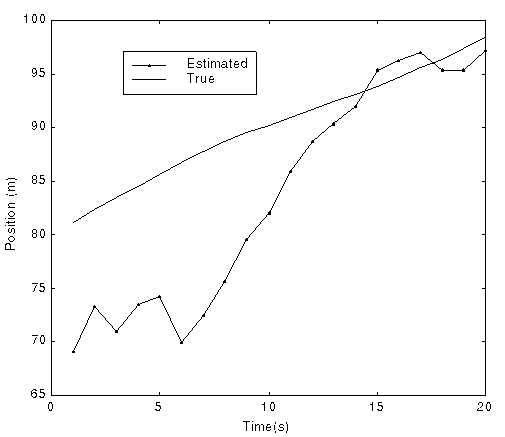
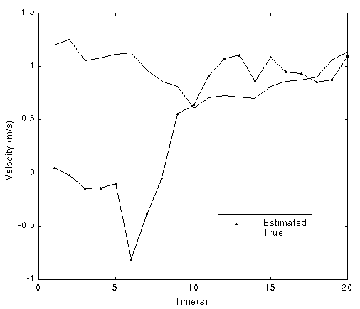
No meaningful result can be derived via single run. Both filters appear to converge (Fig. 1-2) in the sense that the estimation errors tend to decrease.
At least 100 Monte Carlo runs are needed to compare the RMS position and velocity error. The performance is summarized in the table below.
Table 1. Performance comparison between Kalman filter and EKF
| Filter algorithm | RMS position error |
RMS velocity error | Stability | Consistency (NIS/NEES) | Computa-tional burden |
| Kalman | higher | almost same | better | Almost always NO | lower |
| EKF | lower | almost same | worse | Occasionally YES, most of time NO | higher |
Although Kalman filter with direct measurement conversion adds additional bias term to the measurement, the performance seems good without any debiasing approach. The estimation accuracy increases when the angle between the platform and the target increases.
Ī¦ Comparison between linearized filter and nonlinear filter
For the linearized filter, we implement EKF as above. The nonlinear filter estimates the pdf of system's state conditioned on all available measurements using grid approach. The comparison is based on uniform grid with 50 grid points for each state.
Table 2. Performance comparison between linearized filter and nonlinear filter
| Filter algorithm | RMS position error |
RMS velocity error | Stability | Consistency (NIS/NEES) | Computa-tional burden |
| EKF | slightly higher | almost same | better | Occasionally YES, most of time NO | lower |
| nonlinear | slightly lower | almost same or even worse | worse | --------------- | Much higher |
Nonlinear filter does not yields better performance than EKF for the following reasons:
- Moment matching of the measurement noise is not accurate enough.
- The prior pdf has a large deviation from the true pdf in mean and variance.
- The integration procedure at each grid interval uses only approximation which leads to the inaccuracy of conditional mean (the estimator).
- The number of grid is not large enough and the support of the pdf is finite.
Ī¦ Implementation issues of nonlinear estimation
The support of the pdf can be fixed or dynamically changed to the Ī└ 3s region of the previously estimated pdf, the performance does not improve significantly.
If the update integral yields 0 at some time k, the previous pdf does not update (something like gate of the measurement).
The integral taken at each region (consisting of the intervals in position and velocity) of the grid is approximated by assuming that the estimated pdf has a uniformly distributed density function within the small region to be integrated.
The grid can also be nonuniform. A simple implementation is to take the inverse of the interval proportional to the value of the density at each grid. The new value of the density at each grid is derived using line interpolation within the two adjacent grids. When the number of grid points is fixed, nonlinear estimation using nonuniform grid sometimes deteriorates the performance compared with uniform approach. The estimation accuracy is very sensitive to the support of the pdf.
Ī¦ Open questions for future investigation
� Better analytical model to approximate the measurement noise statistic
� More accurate pdf estimation (parametric?) other than grid approach to overcome the heavy computational burden
� Fast simulation techniques for algorithm comparison


Fig. 1 True and estimated position and velocity in a single run
(Using direct coordinates conversion and Kalman filter)
ĪĪ
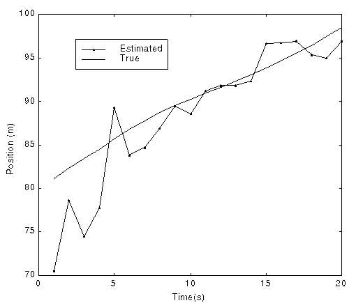
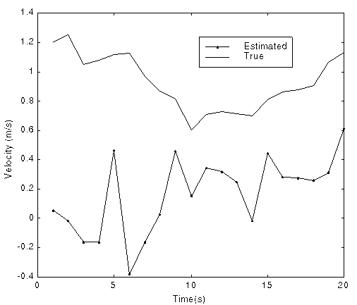
Fig. 2 True and estimated position and velocity in a single run
(Using extended Kalman filter)
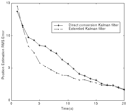
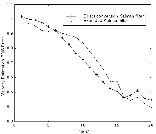
Fig. 3 Comparison of position and velocity estimation RMS errors
(Using Kalman filter with direct coordinates conversion and extended Kalman filter, 100 runs)
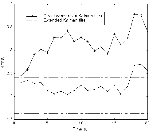
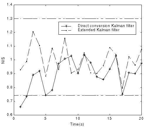
Fig. 4 NEES and NIS with the two-sided 95% probability region
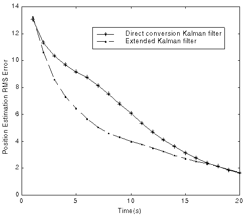
Fig. 5 Comparison of RMS errors between KF and EKF with 1000 runs
(1 out of 1000 diverges for KF, 4 out of 1000 diverge for EKF)
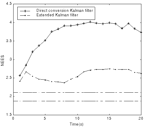
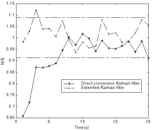
Fig. 6 Comparison of NEES and NIS between KF and EKF with 1000 runs
(with the two-sided 95% probability region for filter consistency check)
ĪĪ
ĪĪ
ĪĪ
ĪĪ
ĪĪ
ĪĪ
ĪĪ
ĪĪ
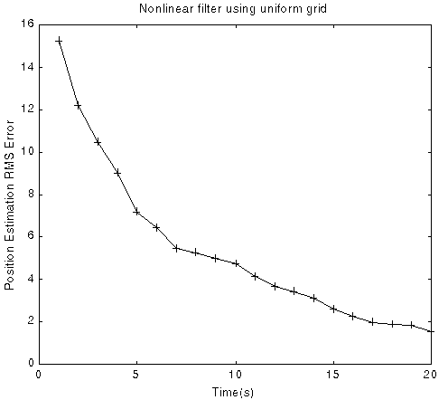
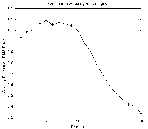
Fig. 7 Position and velocity RMS estimation error
(Using nonlinear estimation with uniform grid, 100 runs)
ĪĪ
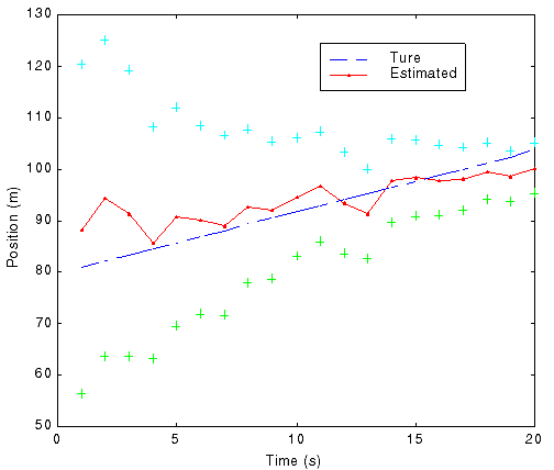
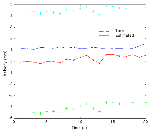
Fig. 8 True and estimated position and velocity in a single run
(Using nonlinear estimation with uniform grid, '+' indicating Ī└ 3s region)
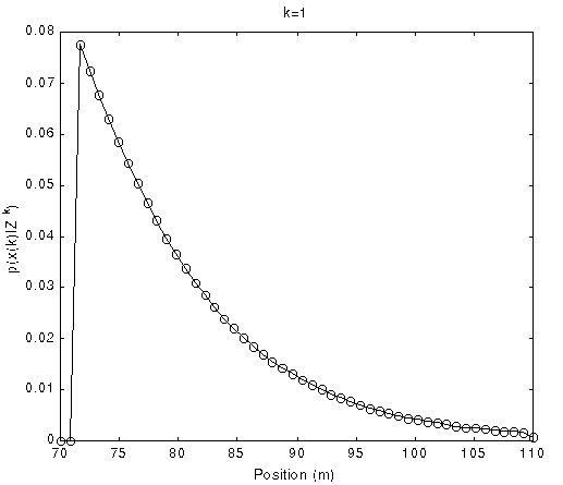
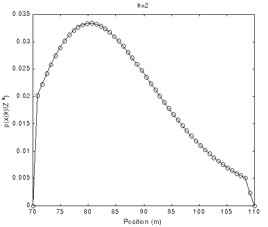
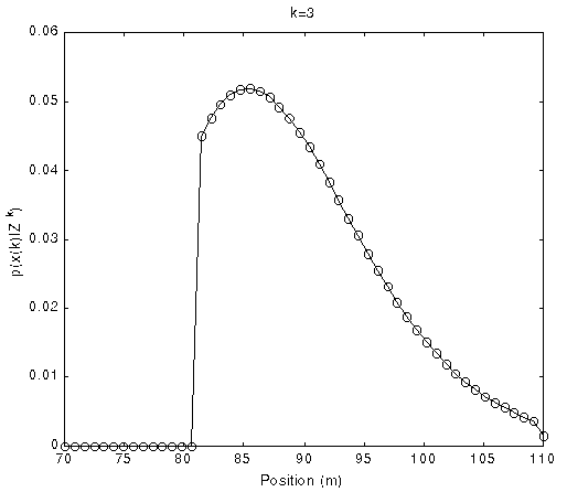
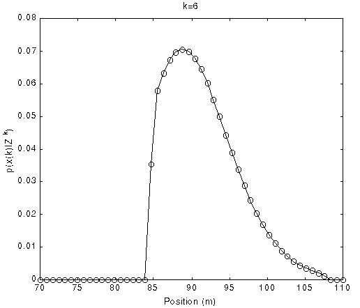
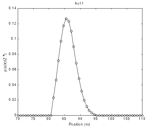
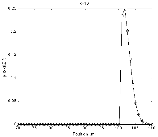
Fig. 9 The PDFs of position with time evolution using uniform grid
(Normalized density function p(x